Code
library(tidyverse)I aim to predict whether an iris flower is of the setosa species based on four numeric features: Sepal.Length, Sepal.Width, Petal.Length, and Petal.Width. These are my independent variables. The dependent variable is a binary factor, IsSetosa, which equals 1 if the flower is a setosa, and 0 otherwise.
Since the dependent variable is binary, I will use logistic regression for this analysis.
library(tidyverse)# Load iris dataset
data(iris)
iris2 <- iris |>
# If setosa, replace with 1. Else replace with 0
mutate(IsSetosa = as.factor(if_else(Species == "setosa", 1, 0))) |>
select(-Species) |>
tibble()
iris2 |> glimpse()Rows: 150
Columns: 5
$ Sepal.Length <dbl> 5.1, 4.9, 4.7, 4.6, 5.0, 5.4, 4.6, 5.0, 4.4, 4.9, 5.4, 4.…
$ Sepal.Width <dbl> 3.5, 3.0, 3.2, 3.1, 3.6, 3.9, 3.4, 3.4, 2.9, 3.1, 3.7, 3.…
$ Petal.Length <dbl> 1.4, 1.4, 1.3, 1.5, 1.4, 1.7, 1.4, 1.5, 1.4, 1.5, 1.5, 1.…
$ Petal.Width <dbl> 0.2, 0.2, 0.2, 0.2, 0.2, 0.4, 0.3, 0.2, 0.2, 0.1, 0.2, 0.…
$ IsSetosa <fct> 1, 1, 1, 1, 1, 1, 1, 1, 1, 1, 1, 1, 1, 1, 1, 1, 1, 1, 1, …# Fit logistic regression
model <- glm(IsSetosa ~ Sepal.Length + Sepal.Width + Petal.Length + Petal.Width,
data = iris2, family = binomial)# Predict probabilities
pred_probs <- predict(model, type = "response")
# Convert probabilities to class labels using 0.5 threshold
pred_classes <- ifelse(pred_probs >= 0.5, 1, 0)# Create confusion matrix
conf_matrix <- table(Predicted = pred_classes, Actual = iris2$IsSetosa)
conf_matrix Actual
Predicted 0 1
0 100 0
1 0 50# Extract values from the confusion matrix
TP <- sum(pred_classes == 1 & iris2$IsSetosa == 1)
FP <- sum(pred_classes == 1 & iris2$IsSetosa == 0)
FN <- sum(pred_classes == 0 & iris2$IsSetosa == 1)
# Calculate precision and recall
precision <- TP / (TP + FP)
recall <- TP / (TP + FN)# Print metrics
cat("Precision:", round(precision, 2), "\n")Precision: 1 cat("Recall:", round(recall, 2), "\n")Recall: 1 Both precision and recall are equal to 1, indicating that the model made no false positives or false negatives when identifying setosa flowers.
summary(model)
Call:
glm(formula = IsSetosa ~ Sepal.Length + Sepal.Width + Petal.Length +
    Petal.Width, family = binomial, data = iris2)

Coefficients:
               Estimate Std. Error z value Pr(>|z|)
(Intercept)     -16.946 457457.097       0        1
Sepal.Length     11.759 130504.042       0        1
Sepal.Width       7.842  59415.385       0        1
Petal.Length    -20.088 107724.594       0        1
Petal.Width     -21.608 154350.616       0        1

(Dispersion parameter for binomial family taken to be 1)

    Null deviance: 1.9095e+02  on 149  degrees of freedom
Residual deviance: 3.2940e-09  on 145  degrees of freedom
AIC: 10

Number of Fisher Scoring iterations: 25
The table above displays the regression coefficients, their standard errors, z-values, and p-values. In logistic regression, R-squared is not directly available, but I can look at the null deviance and residual deviance to assess model fit. A significant drop in deviance suggests a better fit.
exp(coef(model)) (Intercept) Sepal.Length Sepal.Width Petal.Length Petal.Width
4.370970e-08 1.279271e+05 2.544216e+03 1.887509e-09 4.129688e-10 # List of variable names
features <- c("Sepal.Length", "Sepal.Width", "Petal.Length", "Petal.Width")
# Create a named list of ggplot objects
plots <- map(features, function(var) {
ggplot(iris, aes_string(x = var, fill = "Species")) +
geom_density()+
facet_wrap(~Species, ncol = 1, scales = "free_y")+
theme(
axis.title.y = element_blank(),
axis.text.y = element_blank(),
axis.ticks.y = element_blank()
)
}) |>
set_names(features) # Give each plot a name
library(patchwork)
((plots[[1]] + plots[[2]]) / (plots[[3]] + plots[[4]]) +
plot_annotation("Iris Feature Distributions by Species"))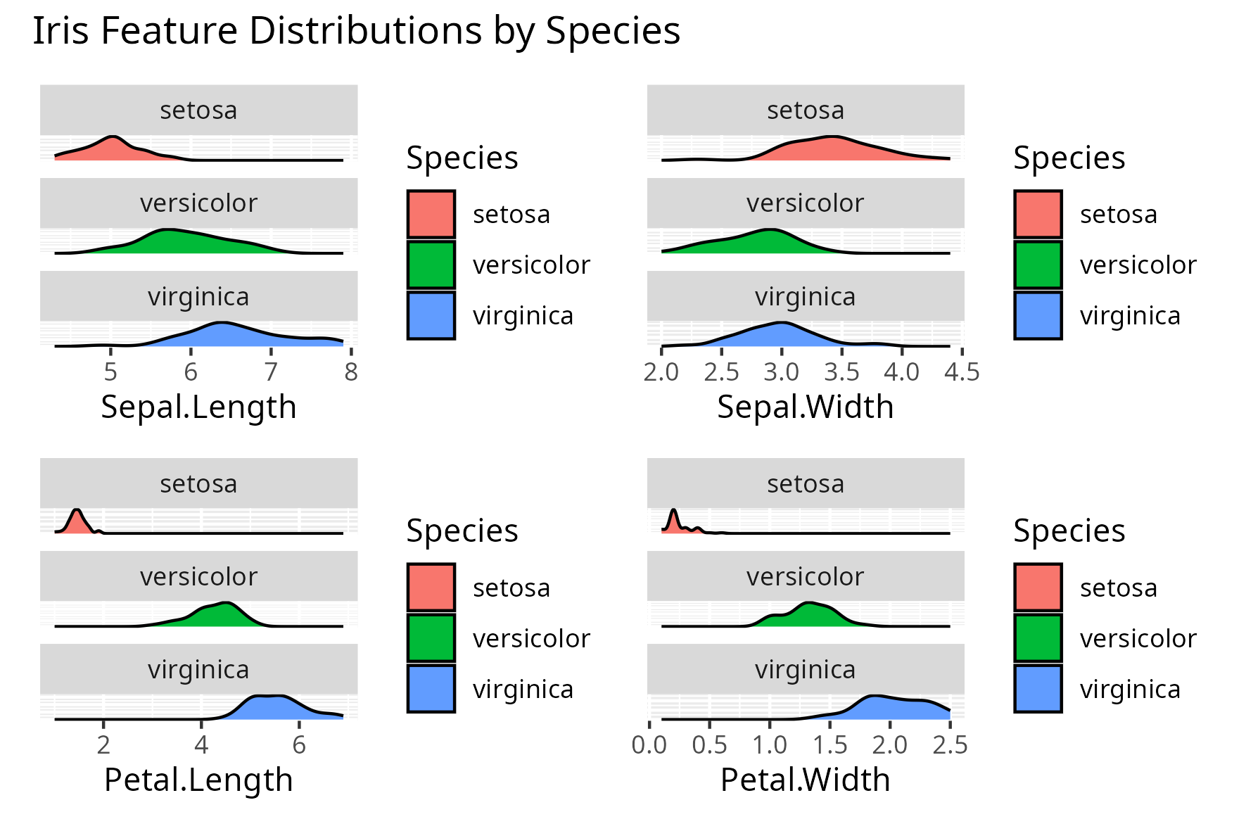
After examining the distribution of each feature by species and converting the model’s coefficients to odds ratios using exp(coef(model)), the following can be said:
Sepal.Length (odds ratio ≈ 1.28e+05)
This suggests that higher sepal length increases the odds of being setosa, which is not fully consistent with the visualization.
In the plot, setosa sepal lengths are actually shorter on average. This contradiction between the odds ratio and the plot likely stems from the logistic regression model assigning relatively low importance to this feature compared to the others.
Sepal.Width (odds ratio ≈ 2.54e+03)
A higher sepal width increases the odds of being setosa, which is somewhat supported by the plot.
Setosa generally shows slightly wider sepals compared to the other species.
Petal.Length (odds ratio ≈ 1.89e-09)
The odds of a flower being setosa decrease sharply as petal length increases.
This is clearly supported by the density plot: setosa has distinctly short petals with little overlap with the other species.
Petal.Width (odds ratio ≈ 4.13e-10)
Like petal length, an increase in petal width dramatically reduces the odds of being setosa.
The plot shows setosa petal widths are very small compared to versicolor and virginica.
(Intercept) (odds ratio ≈ 4.37e-08)
This represents the baseline odds of being setosa when all predictors are 0, which is not meaningful in this context, since 0 is not a realistic value for the input features.
However, the very low value does reflect the fact that setosa makes up only 1/3 of the dataset, so the model starts with low baseline odds of a flower being setosa.
The logistic regression model was able to perfectly classify all observations as either setosa or not, achieving both precision = 1 and recall = 1. This means the model made no false positives or false negatives, correctly identifying all setosa flowers in the dataset.
The model’s success is largely due to the distinctiveness of petal features: setosa has clearly shorter and narrower petals than the other two species, making separation straightforward. While sepal measurements contributed to the model, their effects were less clear and may be influenced by multicollinearity.
In summary, this logistic model performs exceptionally well on this dataset, but caution should be taken when generalizing it beyond the well-behaved and perfectly labeled Iris dataset.
Thumbnail icon from Freepik