Pro Trader RL: A Replication & Extension
Pro Trader RL: A Replication & Extension
A from-scratch implementation and extension of Jeong & Gu (2024)’s Pro Trader RL framework for automated single-ticker stock trading. Two novel contributions, action masking and risk-aware reward shaping, were designed, implemented, and evaluated against the paper’s baseline on SPY and QQQ.
Paper Reference
Da Woon Jeong and Yeong Hyeon Gu. Pro Trader RL: Reinforcement learning framework for generating trading knowledge by mimicking the decision-making patterns of professional traders. Expert Systems with Applications, Volume 254, 2024, Article 124465. https://doi.org/10.1016/j.eswa.2024.124465
Resources
- Datasets: Daily OHLCV bars for SPY (S&P 500 ETF) and QQQ (Nasdaq-100 ETF) from Yahoo Finance via the
yfinancePython package, covering the paper’s test window 2017-10-16 to 2023-10-15. - Libraries used:
numpy,pandas,matplotlib,yfinance,torch(PPO networks),gymnasium(environment scaffolding).
Application, MDP, and RL Model
Application Introduction
The application is automated single-ticker stock trading modeled after the decision process of a professional human trader. The agent observes daily market data, decides whether to enter or exit a position, and accumulates portfolio value over time. The paper’s framework is built around the observation that real traders separate buying decisions from selling decisions because they have different mental models for “is this a good entry?” versus “is this a good moment to exit a position I already own?”. The framework reflects this by using two independent PPO agents instead of a single monolithic one.
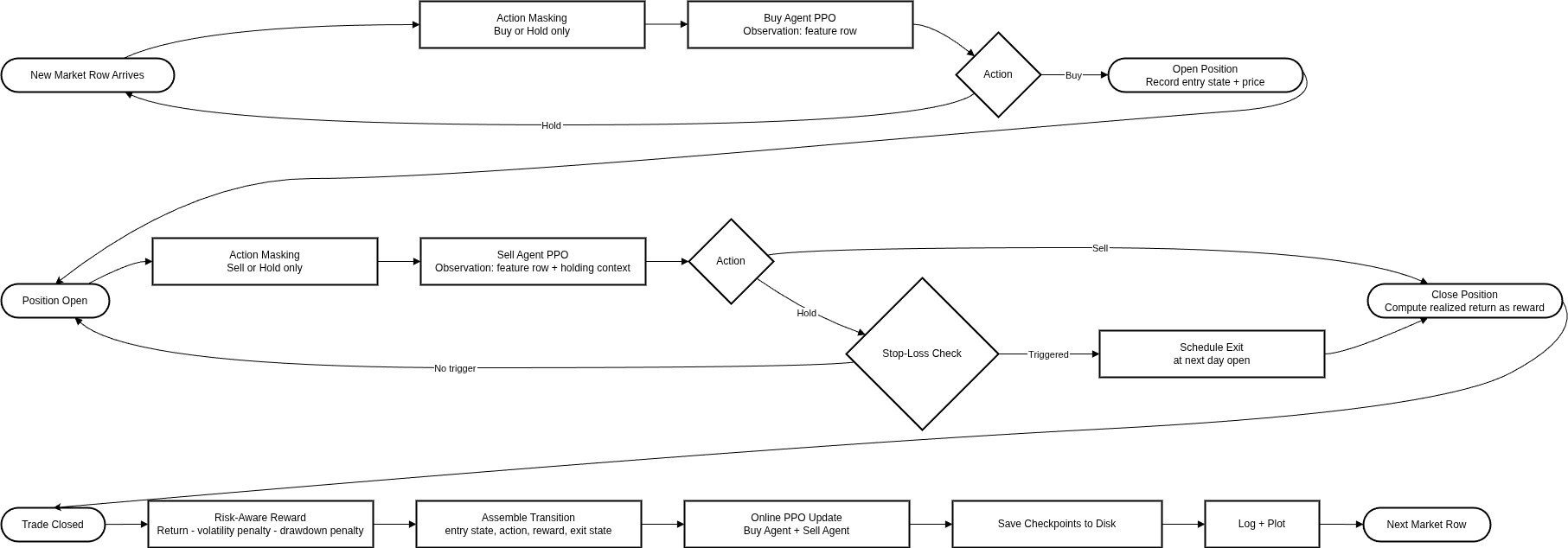
RL agent to environment interface. The codebase implements the environment as a row-by-row data feed. On each trading day, the runner:
- Reads the next OHLCV row from the dataset.
- Builds the state vector (technical indicators + current portfolio status).
- Asks the buy agent if no position is open, or asks the sell agent + stop-loss module if a position is open.
- Executes the chosen action, updates cash and shares, applies the trading fee.
- Logs the transition for downstream PPO updates (online learning every N trades).
This loop runs continuously and supports cancel-and-resume. The runner checkpoints its state after every cycle, so a stopped run resumes exactly where it left off without re-training or re-feeding any data.
Dataset format. Each ticker’s data is a pandas.DataFrame with columns [Open, High, Low, Close, Volume], indexed by trading-day date. The feature pipeline derives 25 indicators on top of these: returns, 10-day and 20-day SMAs, RSI, rolling volatility, Donchian upper/lower channels, breakout signals, trend indicator, and momentum. Features are computed with strict no-look-ahead. Every value at row t uses only data from rows up to and including t.
MDP Formulation
The framework defines two distinct MDPs, one per agent.
Buy MDP.
- State \(s_t\): feature vector at time \(t\): 25-dimensional, containing technical indicators plus a position flag (always 0 here since the buy agent only acts when no position is held).
- Action space \(\mathcal{A}_{\text{buy}} = \{\text{hold}, \text{buy}\}\): discrete, size 2.
- Transition \(P(s_{t+1} | s_t, a_t)\): deterministic given the next row of historical data, since the market is exogenous. The agent’s action only affects the portfolio state, not the price process.
- Reward \(R_t\): for the buy agent, \(R_t = \text{position}_t \cdot (P_{t+1} - P_t)\), i.e., one-step mark-to-market change. The reward is zero on hold, and equal to the next-day price delta on buy. With the risk-aware reward extension, the per-trade reward at exit becomes \(R = \frac{P_{\text{exit}} - P_{\text{entry}}}{P_{\text{entry}}} - \lambda_\sigma\,\sigma\), where \(\sigma\) is the standard deviation of intra-trade returns and \(\lambda_\sigma\) is a tunable penalty weight.
- Discount factor \(\gamma = 0.99\): same as the paper.
Sell MDP. Identical state space. Action space is \(\{\text{hold}, \text{sell}\}\). The reward function in the paper ranks 120-day forward returns from a buy point and assigns scaled rewards based on which return the sell action targets. A simplified version is used: reward = realized return at sell, zero on hold (with the same risk-aware extension applied at exit).
Why this MDP formulation. The paper argues, and it was borne out in the codebase, that combining buy and sell into a single 3-action \(\{\text{buy}, \text{sell}, \text{hold}\}\) policy is hard to train because the same network has to learn two qualitatively different decisions. Splitting them into two MDPs lets each agent’s reward signal stay focused. The trade-off is operational: the runner needs explicit logic to route each decision to the correct agent.
Intuition for value/Q-values. \(Q_{\text{buy}}(s, \text{buy})\) approximates “the expected discounted profit from opening a long position right now and trading optimally afterward.” \(Q_{\text{buy}}(s, \text{hold})\) approximates “the expected discounted profit from staying flat and looking for a better entry later.” The sign of the difference tells the agent whether to enter. Concretely, in the SPY runs the difference tended to be slightly negative throughout most of the test window, explaining why the agent under-traded and underperformed buy-and-hold.
RL Approach
Both buy and sell agents use Proximal Policy Optimization (PPO) in actor-critic form, matching the paper. The actor outputs a softmax distribution over the two actions; the critic outputs a scalar value estimate. Both networks share input features but have separate hidden layers and output heads.
How classical PPO is modified:
- Two-agent split with separate replay buffers. Each agent is updated independently, on its own collected transitions.
- [Innovation] Action masking. Before sampling from \(\pi_\theta\), the logits of structurally invalid actions are set to \(-\infty\):
\[ \tilde{z}_\theta(s)_a = \begin{cases} z_\theta(s)_a & m_a(s) = 1 \\ -\infty & m_a(s) = 0 \end{cases} \]
For the buy agent, “buy” is masked when cash is insufficient to afford one share at the current price plus the 0.1% fee. For the sell agent, “sell” is masked when no position is open. This guarantees the policy never assigns probability mass to actions the environment would silently reject.
- [Innovation] Risk-aware reward. The per-trade reward at exit subtracts a volatility penalty:
\[ R = \frac{P_{\text{exit}} - P_{\text{entry}}}{P_{\text{entry}}} - \lambda_\sigma\,\sigma \]
Setting \(\lambda_\sigma = 0\) recovers the paper’s reward exactly.
- Online updates. PPO updates fire every \(N\) completed trades during the continuous run, instead of only at the end of an episode. This is what the paper calls “online learning” and what this project implements.
Why PPO is appropriate. The action space is small and discrete, the state space is continuous and moderate-dimensional, and the reward signal is sparse (only delivered at trade exits). PPO’s clipped objective handles the high-variance gradients that come from sparse rewards more gracefully than vanilla policy gradient or A2C. The paper compares against both DQN and A2C baselines and reports PPO outperforming both in this setting; those baselines were not re-run but their conclusion was adopted.
Architecture diagram. The figure below shows the per-row continuous trading loop, with both PPO agents, the action masking step, the stop-loss check, and the risk-aware reward update.
Codebase, System, and Experiment Setup
Libraries and System Setup
Python version: 3.12.11
Setup steps:
# Install required packages
pip install pandas yfinance pyarrow fastparquet numpy matplotlib torch gymnasium

# Download data (writes parquet files into data/raw)
python scripts/download_data.py

# Build the feature dataset
python scripts/build_dataset.py
Running Experiments
The primary entry point is run_continuous_trader.py, which takes a JSON config file:
python scripts/run_continuous_trader.py configs/default.jsonSwitching between configurations. The runtime config controls every experiment-relevant flag. The relevant fields are:
| Field | Effect |
|---|---|
data.ticker |
"SPY" or "QQQ" (or any other Yahoo Finance symbol) |
runtime.action_masking |
true or false; toggles innovation 1 |
reward.risk_aware.lambda_sigma |
volatility penalty weight (0.0 recovers paper reward) |
reward.regime_aware.enabled |
true enables regime-conditional weighting (innovation extension) |
Running all four core experiments:
# Exp 1: SPY, no innovations
python scripts/run_continuous_trader.py configs/exp1_spy_baseline.json

# Exp 2: QQQ, no innovations
python scripts/run_continuous_trader.py configs/exp2_qqq_baseline.json

# Exp 3: SPY, both innovations
python scripts/run_continuous_trader.py configs/exp3_spy_innov.json

# Exp 4: QQQ, both innovations
python scripts/run_continuous_trader.py configs/exp4_qqq_innov.json
The regime-conditional extension experiments (Exp 5 and 6) use the same runner with reward.regime_aware.enabled = true.
Experiments
Replication Experiment 1: Pro Trader RL Framework on a Single-Ticker Setup
Purpose and setup. Reproduce the structure and outcome direction of the paper’s Experiment 1 (Table 7) on a single-ticker setup. The paper trains across 1,465 stocks; this experiment restricts to SPY (broad-market ETF) and QQQ (Nasdaq-100 ETF) as the two universes. The test window matches the paper exactly: 2017-10-16 to 2023-10-15.
Four configurations are run:
- Exp 1: SPY, no innovations.
- Exp 2: QQQ, no innovations.
- Exp 3: SPY, with action masking and risk-aware reward.
- Exp 4: QQQ, with action masking and risk-aware reward.
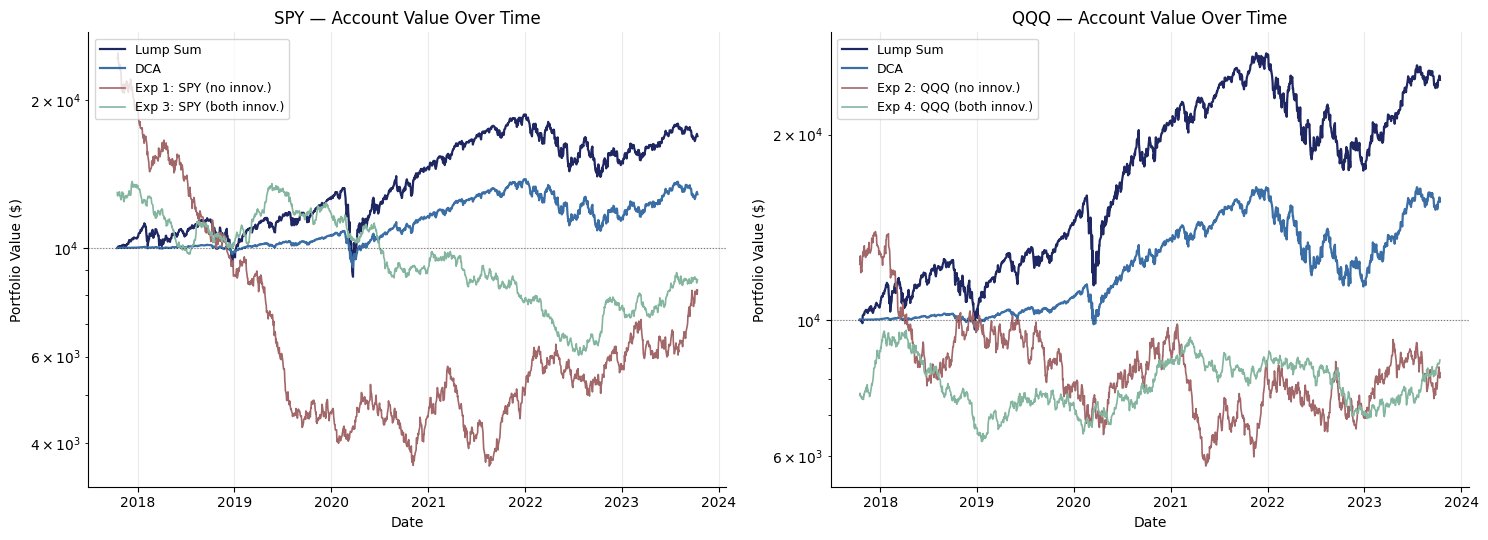
Two passive benchmarks are calculated alongside each ticker for context:
- Lump Sum: buy as many shares as $10,000 affords on day 1, hold to the end.
- DCA (Dollar-Cost Average): invest the $10,000 in equal monthly slices across the test window.
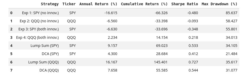
How to read the results. Four metrics, all in percent except Sharpe:
- Annual Return: geometric annualization of total return over the test window. Higher is better.
- Cumulative Return: total fractional return from start to end. Higher is better.
- Sharpe Ratio: mean daily return divided by daily-return standard deviation, scaled by \(\sqrt{252}\). Higher is better.
- Max Drawdown (MDD): worst peak-to-trough fractional drop over the period. Lower is better.
Account value over time.
Per-strategy summary table.
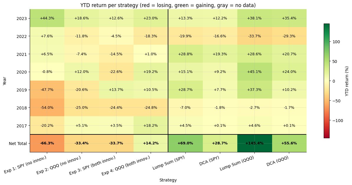
Year-by-year heatmap. Reading the heatmap top-to-bottom shows how each strategy performed in each calendar year of the test window; the bottom row aggregates net total return across the full window.
Retrospective: What Went Wrong and What I Learned
The RL agent didn’t beat buy-and-hold or dollar cost averaging. The paper’s results on 1,465 stocks didn’t transfer cleanly to a single-ticker setup, and I ran into a lot of issues along the way. But through those issues, I gained first-hand experience with the struggles of RL.
Problems I encountered:
- Always-buy collapse. The agent would learn to just buy and never sell, essentially becoming a worse version of buy-and-hold (worse because it paid trading fees on entry). This took a while to debug and required splitting the buy and sell agents more carefully.
- Sparse reward signals. With reward only delivered at trade exits, the policy gradients were high-variance and training was unstable. The risk-aware reward helped but didn’t fully solve it.
- Two-agent coordination. Routing decisions between two independent PPO agents sounds clean in theory but introduced subtle bugs. The buy agent would sometimes try to act while a position was open because the state masking wasn’t wired correctly.
- Single-ticker limitation. The paper’s framework was designed for 1,465 stocks simultaneously, which creates natural diversification and more training signal. On a single ticker, the agent sees far fewer trades and has less opportunity to learn.
- Hyperparameter sensitivity. Small changes in the PPO clipping parameter, learning rate, or the risk penalty weight \(\lambda_\sigma\) produced wildly different behaviors. Finding stable configurations was trial-and-error heavy.
- Online learning complexity. Updating the policy mid-run instead of after full episodes meant the agent could unlearn things it had just figured out. The checkpointing system was essential for recovering from bad update cycles.
What I took away from this:
This project taught me more than a successful one would have. I got hands-on experience with MDP formulation, PPO implementation, debugging policy collapse, building custom Gymnasium environments, and designing reward functions that actually shape behavior. I also learned that replicating reinforcement learning papers is harder than it looks. The gap between a paper’s methodology section and a working codebase is wide, and closing that gap requires understanding the material at a much deeper level than just reading it.
I would approach a project like this differently now. I would start with a simpler environment, validate the PPO implementation against a known baseline like CartPole, then gradually add complexity. I would also test on synthetic data with known structure before using real market data. But working through the failures gave me a realistic sense of what RL can and cannot do in financial settings, and that is more valuable than a polished result.
Thumbnail icon from Freepik